Sometimes debuggers and profilers are obviously broken, sometimes it's subtle and hard to spot. From my flame graphs page:

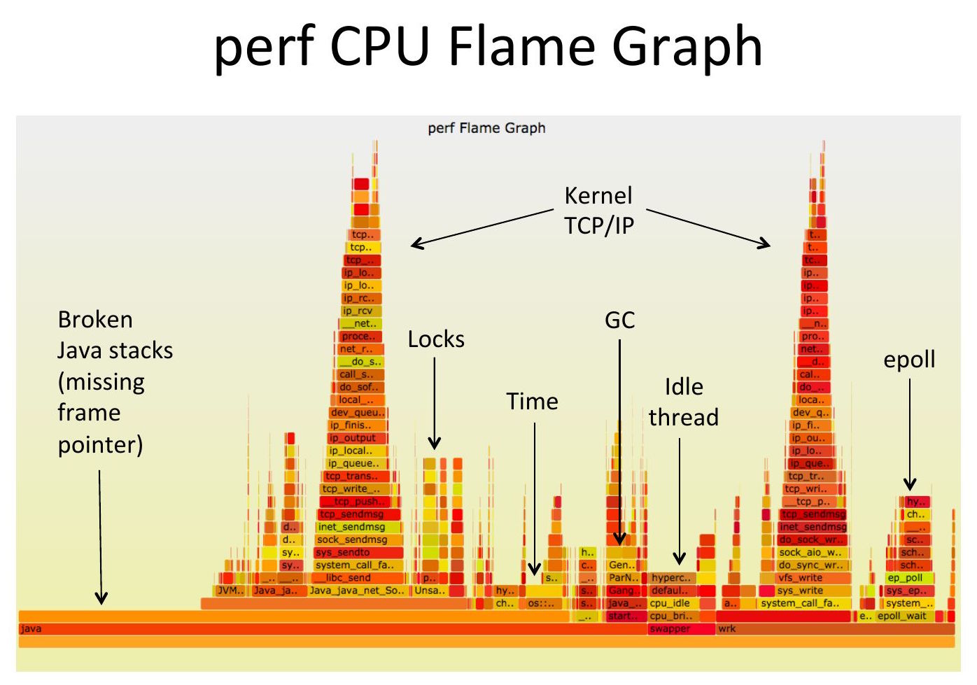
CPU flame graph (partly broken)

(Click for original SVG.) This is pretty common and usually goes unnoticed as the flame graph looks ok at first glance. But there are 15% of samples on the left, above "[unknown]", that are in the wrong place and missing frames. The problem is that this system has a default libc that has been compiled without frame pointers, so any stack walking stops at the libc layer, producing a partial stack that's missing the application frames. These partial stacks get grouped together on the left.

Other types of profiling hit this more often. Off-CPU flame graphs, for example, can be dominated by libc read/write and mutex functions, so without frame pointers end up mostly broken. Apart from library code, maybe your application doesn't have frame pointers either, in which case everything is broken.

I'm posting about this problem now because Fedora and Ubuntu are releasing versions that fix it, by compiling libc and more with frame pointers by default. This is great news as it not only fixes these flame graphs, but makes off-CPU flame graphs far more practical. This is also a win for continuous profilers (my employer, Intel, just announced one) as it makes customer adoption easier.

What are frame pointers?

The x86-64 ABI documentation shows how a CPU register, %rbp, can be used as a "base pointer" to a stack frame, aka the "frame pointer." I pictured how this is used to walk stack traces in my BPF book.

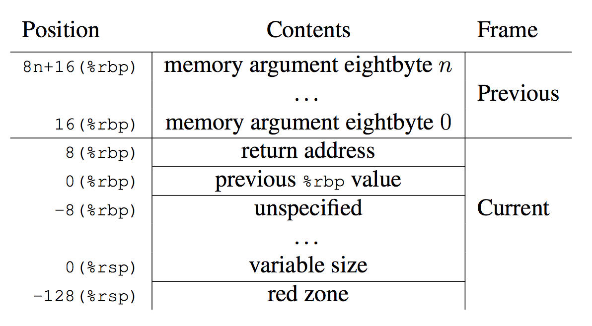
Figure 3.3: Stack Frame with Base Pointer (x86-64 ABI)

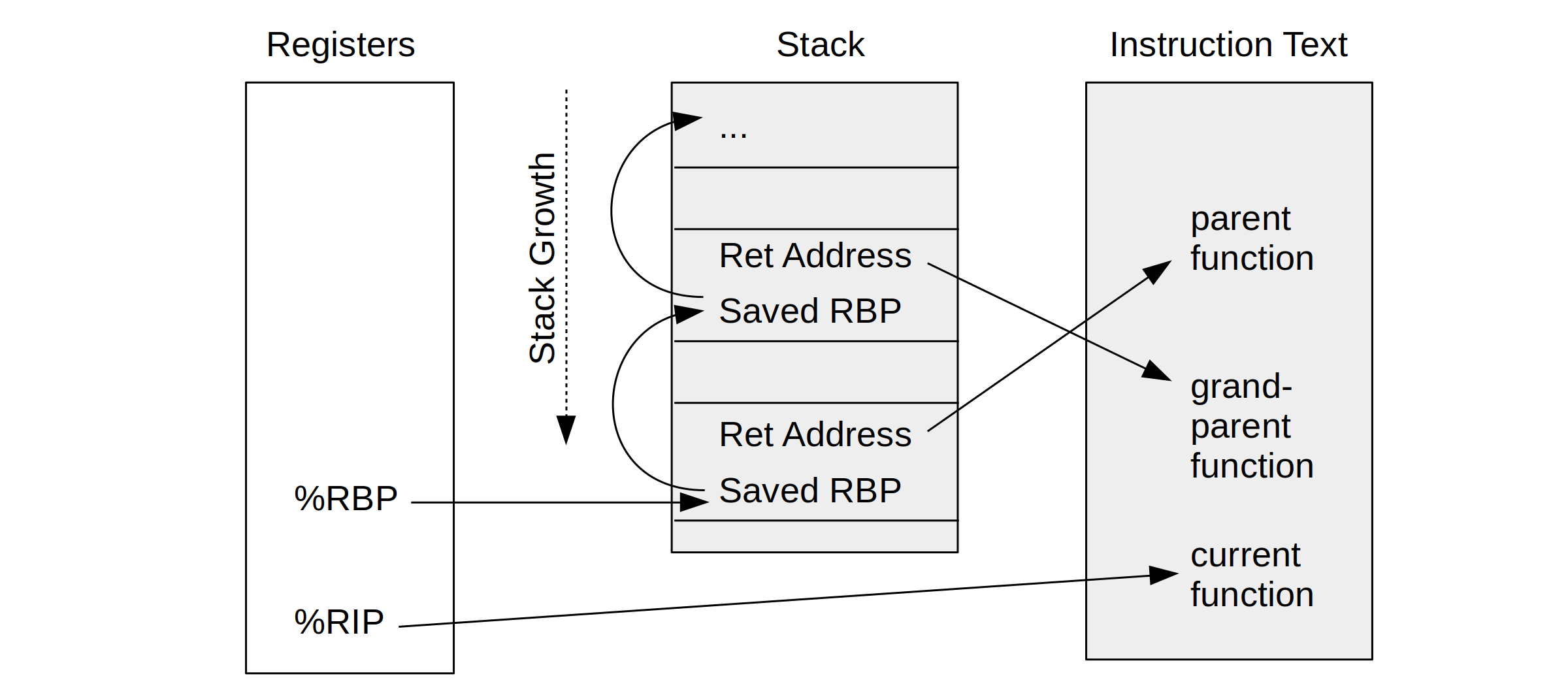
Figure 2-6: Frame Pointer-based Stack Walking (BPF book)

This stack-walking technique is commonly used by external profilers and debuggers, including Linux perf and eBPF, and ultimately visualized by flame graphs. However, the x86-64 ABI has a footnote [12] to say that this register use is optional:

"The conventional use of %rbp as a frame pointer for the stack frame may be avoided by using %rsp (the stack pointer) to index into the stack frame. This technique saves two instructions in the prologue and epilogue and makes one additional general-purpose register (%rbp) available."

(Trivia: I had penciled the frame pointer function prologue and epilogue on my Netflix office wall, lower left.)

2004: Their removal

In 2004 a compiler developer, Roger Sayle, changed gcc to stop generating frame pointers, writing:

"The simple patch below tweaks the i386 backend, such that we now default to the equivalent of "-fomit-frame-pointer -ffixed-ebp" on 32-bit targets"

i386 (32-bit microprocessors) only have four general purpose registers, so freeing up %ebp takes you from four to five (or if you include %si and %di, from six to seven). I'm sure this delivered large performance improvements and I wouldn't try arguing against it. Roger cited two other reasons for this change: The desire to outperform Intel's icc compiler, and the belief that it didn't break debuggers (of the time) since they supported other stack walking techniques.

2005-2023: The winter of broken profilers

However, the change was then applied to x86-64 (64-bit) as well, which had over a dozen registers and didn't benefit so much from freeing up one more. And there are debuggers/profilers that this change did break (typically system profilers, not language specific ones), more so today with eBPF, which didn't exist back then. As my former Sun Microsystems colleague Eric Schrock (nickname Schrock) wrote in November 2004:

"On i386, you at least had the advantage of increasing the number of usable registers by 20%. On amd64, adding a 17th general purpose register isn't going to open up a whole new world of compiler optimizations. You're just saving a pushl, movl, an series of operations that (for obvious reasons) is highly optimized on x86. And for leaf routines (which never establish a frame), this is a non-issue. Only in extreme circumstances does the cost (in processor time and I-cache footprint) translate to a tangible benefit - circumstances which usually resort to hand-coded assembly anyway. Given the benefit and the relative cost of losing debuggability, this hardly seems worth it."

In Schrock's conclusion:

"it's when people start compiling /usr/bin/ without frame pointers that it gets out of control."

This is exactly what happened on Linux, not just /usr/bin but also /usr/lib and application code! I'm sure there are people who are too new to the industry to remember the pre-2004 days when profilers would "just work" without OS and runtime changes.

2014: Java in Flames

Broken Java Stacks (2014)

When I joined Netflix in 2014, I found Java's lack of frame pointer support broke all application stacks (pictured in my 2014 Surge talk on the right). I ended up developing a fix for the JVM c2 compiler which Oracle reworked and added as the -XX:+PreserveFramePointer option in JDK8u60 (see my Java in Flames post for details [PDF]).

While that Java change led to discovering countless performance wins in application code, libc was still breaking some portion of the samples (as pictured in the example at the top of this post) and was breaking most stacks in off-CPU flame graphs. I started by compiling my own libc for production use with frame pointers, and then worked with Canonical to have one prebuilt for Ubuntu. For a while I was promoting the use of Canonical's libc6-prof, which was libc6 with frame pointers.

2015-2020: Overhead

As part of production rollout I did many performance overhead tests, which I've described publicly before: The overhead of adding frame pointers to everything (libc and Java) was usually less than 1%, with one exception of 10%. That 10% was an unusual application that was generating stack traces over 1000 frames deep (via Groovy), so deep that it broke Linux's perf profiler. Arnaldo Carvalho de Melo (Red Hat) added the kernel.perf_event_max_stack sysctl just for this Netflix workload. It was also a virtual machine that lacked low-level hardware profiling capabilities, so I wasn't able to do cycle analysis to confirm that the 10% was entirely frame pointer-based.

The actual overhead depends on your workload. Others have reported around 1% and around 2%. Microbenchmarks can be the worst, hitting 10%: This doesn't surprise me since they resolve to running a small funciton in a loop, and adding any instructions to that function can cause it to spill out of L1 cache warmth (or cache lines) causing a drop in performance. If I were analyzing such a microbenchmark, apart from observability anaylsis (cycles, instructions, PMU, PMCs, PEBS) there is also an experiment I'd like to try:

To test the theory of I-cache spillover: Compile the microbenchmark with and without frame pointers and find the performance delta. Then flame graph the microbenchmark to understand the hot function. Then add some inline assembly to the hot function where you add enough NOPs to the start and end to mimic the frame pointer prologue and epilogue (I recommend writing them on your office wall in pencil), compile it without frame pointers, disassemble the compiled binary to confirm those NOPs weren't stripped, and now test that. If the performance delta is still large (10%) you've confirmed that it is due to cache effects, and anyone who was worked at this level in production will tell you that it's the straw that broke the camel's back. Don't blame the straw, in this case, the frame pointers. Adding anything will cause the same effect. Having done this before, it reminds me of CSS programming: you make a little change here and everything breaks, and you spend hours chasing your own tail.

Another extreme example of overhead was the Python scimark_sparse_mat_mult benchmark, which could reach 10%. Fortunately this was analyzed by Andrii Nakryiko (Meta) who found it was a unusual case of a large function where gcc switched from %rsp offsets to %rbp-relative offsets, which took more bytes to store, causing performance issues. I've heard this has since been fixed so that Python can reenable frame pointers by default.

As I've seen frame pointers help find performance wins ranging from 5% to 500%, the typical "less than 1%" cost (or even 1% or 2% cost) is easily justified. But I'd rather the cost be zero, of course! We may get there with future technologies I'll cover later. In the meantime, frame pointers are the most practical way to find performance wins today.

What about Linux on devices where there is no chance of profiling or debugging, like electric toothbrushes? (I made that up, AFAIK they don't run Linux, but I may be wrong!) Sure, compile without frame pointers. The main users of this change are enterprise Linux. Back-end servers.

2022: Upstreaming, first attempt

Other large companies with OS and perf teams (Meta, Google) hinted strongly that they had already enabled frame pointers for everything years earlier. (Google should be no surprise because they pioneered continuous profiling.) So at this point you had Google, Meta, and Netflix running their own libc with frame pointers and able to enjoy profiling capabilities that most other companies – without dedicated OS teams – couldn't get working. Can't we just upstream this so everyone can benefit?

There's a bunch of difficulties when taking "works well for me" changes and trying to make them the default for everyone. Among the difficulties is that end-user companies don't have a clear return on the investment from telling their Linux vendor what they fixed, since they already fixed it. I guess the investment is quite small, we're talking about a single email, right?...Wrong! Your suggestion is now a 116-post thread where everyone is sharing different opinions and demanding this and that, as we found out the hard way. For Fedora, one person requested:

"Meta and/or Netflix should provide infrastructure for a side repository in which the change can be tested and benchmarked and the code size measured."

(Bear in mind that Netflix doesn't even use Fedora!)

Jonathan Corbet, who writes the best Linux articles, summarized this in "Fedora's tempest in a stack frame" which is so detailed that I feel PTSD when reading it. It's good that the Fedora community wants to be so careful, but I'd rather spend time discussing building something better than frame pointers, perhaps involving ORC, LBR, eBPF, and other technologies, than so much worry about looking bad in kitchen-sink benchmarks that I wouldn't trust in the first place.

2023, 2024: Frame Pointers in Fedora and Ubuntu!

Fedora revisited the proposal and has accepted it this time, making it the first distro to reenable frame pointers. Thank you!

Ubuntu has also announced frame pointers by default in Ubuntu 24.04 LTS. Thank you!

UPDATE: I've now heard that Arch Linux is also enabling frame pointers! Thanks Daan De Meyer (Meta).

While this fixes stack walking through OS libraries, you might find your application still doesn't support stack tracing, but that's typically much easier to fix. Java, for example, has the -XX:+PreserveFramePointer option. There were ways to get Golang to support frame pointers, but that became the default years ago. Just to name a couple of languages.

2034+: Beyond Frame Pointers

There's more than one way to walk a stack. These could be separate blog posts, but I want to comment briefly on alternates:

• LBR (Last Branch Record): Intel's hardware feature that was limited to 16 or 32 frames. Most application stacks are deeper, so this can't be used to build flame graphs, but it is better than nothing. I use it as a last resort as it gives me some stack insights.
• BTS (Branch Trace Store): Another Intel thing. Not so limited to stack depth, but has overhead from memory load/stores and BTS buffer overflow interrupt handling.
• AET (Archetectural Event Trace): Another Intel thing. It's a JTAG-based tracer that can trace low-level CPU, BIOS, and device events, and apparently can be used for stack traces as well. I haven't used it. (I spent years as a cloud customer where I couldn't access many HW-level things.) I hope it can be configured to output to main memory, and not just a physical debug port.
• DWARF: Binary debuginfo, has been used forever with debuggers. Update: I'd said it doesn't exist for JIT'd runtimes like the Java JVM, but others have pointed out there has been some JIT->DWARF work done. I still don't expect it to be practical on busy production servers that are constantly in c2. The overhead just to walk DWARF is also high, as it was designed for non-realtime use. Javier Honduvilla Coto (Polar Signals) did some interesting work using an eBPF walker to reduce the overhead, but...Java.
• eBPF stack walking: Mark Wielaard (Red Hat) demonstrated a Java JVM stack walker using SystemTap back at LinuxCon 2014, where an external tracer walked a runtime with no runtime support or help. Very cool. This can be done using eBPF as well. The performmance overhead could be too high, however, as it may mean a lot of user space reads of runtime internals depending on the runtime. It would also be brittle; such eBPF stack walkers should ship with the language code base and be maintained with it.
• ORC (oops rewind capability): The Linux kernel's new lightweight stack unwinder by Josh Poimboeuf (Red Hat) that has allowed newer kernels to remove frame pointers yet retain stack walking. You may be using ORC without realizing it; the rollout was smooth as the kernel profiler code was updated to support ORC (perf_callchain_kernel()->unwind_orc.c) at the same time as it was compiled to support ORC. Can't ORCs invade user space as well?
• SFrames (Stack Frames): ...which is what SFrames does: lightweight user stack unwinding based on ORC. There have been recent talks to explain them by Indu Bhagat (Oracle) and Steven Rostedt (Google). I should do a blog post just on SFrames.
• Shadow Stacks: A newer Intel and AMD security feature that can be configured to push function return addresses onto a separate HW stack so that they can be double checked when the return happens. Sounds like such a HW stack could also provide a stack trace, without frame pointers.
• (And this isn't even all of them.)

Daan De Meyer (Meta) did a nice summary as well of different stack walkers on the Fedora wiki.

So what's next? Here's my guesses:

• 2029: Ubuntu and Fedora release new versions with SFrames for OS components (including libc) and ditches frame pointers again. We'll have had five years of frame pointer-based performance wins and new innovations that make use of user space stacks (e.g., better automated bug reporting), and will hit the ground running with SFrames.
• 2034: Shadow stacks have been enabled by default for security, and then are used for all stack tracing.

Conclusion

I could say that times have changed and now the original 2004 reasons for omitting frame pointers are no longer valid in 2024. Those reasons were that it improved performance significantly on i386, that it didn't break the debuggers of the day (prior to eBPF), and that competing with another compiler (icc) was deemed important. Yes, times have indeed changed. But I should note that one engineer, Eric Schrock, claimed that it didn't make sense back in 2004 either when it was applied to x86-64, and I agree with him. Profiling has been broken for 20 years and we've only now just fixed it.

Fedora and Ubuntu have now returned frame pointers, which is great news. People should start running these releases in 2024 and will find that CPU flame graphs make more sense, Off-CPU flame graphs work for the first time, and other new things become possible. It's also a win for continuous profilers, as they don't need to convince their customers to make OS changes to get profiles to fully work.

Thanks

The online threads about this change aren't even everything, there have been many discussions, meetings, and work put into this, not just for frame pointers but other recent advances including ORC and SFrames. Special thanks to Andrii Nakryiko (Meta), Daan De Meyer (Meta), Davide Cavalca (Meta), Ian Rogers (Google), Steven Rostedt (Google), Josh Poimboeuf (Red Hat), Arjan Van De Ven (Intel), Indu Bhagat (Oracle), Mark Shuttleworth (Canonical), Jon Seager (Canonical), Oliver Smith (Canonical), Javier Honduvilla Coto (Polar Signals), Mark Wielaard (Red Hat), Ben Cotton (Red Hat), and many others (see the Fedora discussions). And thanks to Schrock.

Appendix: Fedora

For reference, here's my writeup for the Fedora change:

I enabled frame pointers at Netflix, for Java and glibc, and summarized the effect in BPF Performance Tools (page 40):

"Last time I studied the performance gain from frame pointer omission in our production environment, it was usually less than one percent, and it was often so close to zero that it was difficult to measure. Many microservices at Netflix are running with the frame pointer reenabled, as the performance wins found by CPU profiling outweigh the tiny loss of performance."

I've spent a lot of time analyzing frame pointer performance, and I did the original work to add them to the JVM (which became -XX:+PreserveFramePoiner). I was also working with another major Linux distro to make frame pointers the default in glibc, although I since changed jobs and that work has stalled. I'll pick it up again, but I'd be happy to see Fedora enable it in the meantime and be the first to do so.  

We need frame pointers enabled by default because of performance. Enterprise environments are monitored, continuously profiled, and analyzed on a regular basis, so this capability will indeed be put to use. It enables a world of debugging and new performance tools, and once you find a 500% perf win you have a different perspective about the <1% cost. Off-CPU flame graphs in particular need to walk the pthread functions in glibc as most blocking paths go through them; CPU flame graphs need them as well to reconnect the floating glibc tower of futex/pthread functions with the developers code frames.

I see the comments about benchmark results of up to 10% slowdowns. It's good to look out for regressions, although in my experience all benchmarks are wrong or deeply misleading. You'll need to do cycle analysis (PEBS-based) to see where the extra cycles are, and if that makes any sense. Benchmarks can be super sensitive to degrading a single hot function (like "CPU benchmarks" that really just hammer one function in a loop), and if extra instructions (function prologue) bump it over a cache line or beyond L1 cache-warmth, then you can get a noticeable hit. This will happen to the next developer who adds code anyway (assuming such a hot function is real world) so the code change gets unfairly blamed. It will only regress in this particular scenario, and regression is inevitable. Hence why you need the cycle analysis ("active benchmarking") to make sense of this.

There was one microservice that was an outlier and had a 10% performance loss with Java frame pointers enabled (not glibc, I've never seen a big loss there). 10% is huge. This was before PMCs were available in the cloud, so I could do little to debug it. Initially the microservice ran a "flame graph canary" instance with FPs for flame graphs, but the developers eventually just enabled FPs across the whole microservice as the gains they were finding outweighed the 10% cost. This was the only noticeable (as in, >1%) production regression we saw, and it was a microservice that was bonkers for a variety of reasons, including stack traces that were over 1000 frames deep (and that was after inlining! Over 3000 deep without. ACME added the perf_event_max_stack sysctl just so Netflix could profile this microservice, as the prior limit was 128). So one possibility is that the extra function prologue instructions add up if you frequently walk 1000 frames of stack (although I still don't entirely buy it). Another attribute was that the microservice had over 1 Gbyte of instruction text (!), and we may have been flying close to the edge of hardware cache warmth, where adding a bit more instructions caused a big drop. Both scenarios are debuggable with PMCs/PEBS, but we had none at the time.

So while I think we need to debug those rare 10%s, we should also bear in mind that customers can recompile without FPs to get that performance back. (Although for that microservice, the developers chose to eat the 10% because it was so valuable!) I think frame pointers should be the default for enterprise OSes, and to opt out if/when necessary, and not the other way around. It's possible that some math functions in glibc should opt out of frame pointers (possibly fixing scimark, FWIW), but the rest (especially pthread) needs them.

In the distant future, all runtimes should come with an eBPF stack walker, and the kernel should support hopping between FPs, ORC, LBR, and eBPF stack walking as necessary. We may reach a point where we can turn off FPs again. Or maybe that work will never get done. Turning on FPs now is an improvement we can do, and then we can improve it more later.

For some more background: Eric Schrock (my former colleague at Sun Microsystems) described the then-recent gcc change in 2004 as "a dubious optimization that severely hinders debuggability" and that "it's when people start compiling /usr/bin/* without frame pointers that it gets out of control" I recommend reading his post: [0].

The original omit FP change was done for i386 that only had four general-purpose registers and saw big gains freeing up a fifth, and it assumed stack walking was a solved problem thanks to gdb(1) without considering real-time tracers, and the original change cites the need to compete with icc [1]. We have a different circumstance today -- 18 years later -- and it's time we updated this change.

[0] http://web.archive.org/web/20131215093042/https://blogs.oracle.com/eschrock/entry/debugging_on_amd64_part_one
[1] https://gcc.gnu.org/ml/gcc-patches/2004-08/msg01033.html

This Development-cycle in Cargo: 1.78

We wanted to share what has been happening for the last 6 weeks to better keep the community informed and involved. For work that was merged before the beta branch was made at the end of the cycle, it will be in the Beta channel for the next 6 weeks after which it will be generally available.

This is distinct from This Week in Rust in that it tries to focus more on the big picture, rather than individual PRs, and pulls from more sources, like Cargo Team meetings and Zulip.

This is an experiment in finding better ways to be engaged with the community and we'll see how well it works and how well we can keep up on it.

• Plugin of the cycle
• Implementation
  • Terminal styling
  • User-controlled diagnostics
  • Performance
  • MSRV-aware Cargo
  • Registry authentication
  • Git extensions
  • Garbage collection
  • Default Edition
  • Open namespaces
• Design discussions
  • Deprecated Cargo.toml fields
  • RFC #3452: Nested packages
  • Why is this yanked?
  • Weak feature syntax
• Misc
• Focus areas without progress

Plugin of the cycle

Cargo can't be everything to everyone, if for no other reason than the compatibility guarantees it must uphold. Plugins play an important part of the Cargo ecosystem and we want to celebrate them.

Our plugin for this cycle is cargo-sweep which removes unused build files. See also cargo-cache. For a related work inside of Cargo, see #12633.

Thanks to LukeMathWalker for the suggestion!

Please submit your suggestions for the next post.

Implementation

Terminal styling

While Cargo has UI tests, they have not verified the terminal styling, like colors. Rustc manages this by writing the ANSI escape codes to text files which are hard to visualize outside of cat stdout.log. In #13461, epage ported Cargo's UI snapshots from text to SVG, allowing terminal styling to be captured. To accomplish this, they created anstyle-svg to render ANSI escape codes as styles in an SVG (credit goes to term-transcript for the original idea) and integrated that into snapbox (trycmd#256) which we use for snapshoting our UI tests.

(not a screenshot but generated from cargo's output)

While this verified most of Cargo's terminal styling, we couldn't force styling on within --help to snapshot it. While we added styling to --help in #12578, we overlooked this being controlled by term.color as this all happens before the config is initialized. In #13463, we refactored Cargo's initialization so at least some config is available before parsing command-line arguments, allowing --help to be controlled by config. This still leaves cargo --color=never --help as unsupported (#9012).

In reviewing the SVG snapshots, we identified some CLI help output that was overlooked in #12578 and addressed it in #13479

Since then, rustc (thanks to estebank in rust#121877) and annotate-snippets (thanks to Muscraft in annotate-snippets-rs#86) have adopted SVG snapshot testing of terminal styling

User-controlled cargo diagnostics

Update from 1.77. In summary, this aims to add user-controlled lints that look like rustc and are controlled through the [lints] table

One problem we had with the SVG snapshot tests was with annotate-snippets, the rustc-like diagnostic renderer that Cargo is using. Rustc, and by extension annotate-snippets, specializes the colors for each platform for maximum compatibility with the default colors used by each platform's most common terminals. To workaround this, we had to put in snapshot wildcards in place of the style names, making the SVGs render different than what you'd get on the terminal. Muscraft added the testing-colors feature to annotate-snippets to force consistent colors across platforms for testing (annotate-snippets-rs#82), allowing us to have the SVGs better match the terminal while working on all platforms.

In preparation to shift our focus from annotate-snippets to Cargo's diagnostic system, we reviewed Cargo's code for generating messages for TOML parsing errors for any cleanup we should first apply to Cargo and/or annotate-snippets. annotate-snippets requires callers to deal with columns but that is a UX concern that is dependent on the medium you are rendering to so Muscraft shifted the API to focus on byte indices (annotate-snippets-rs#90). There is still a lot of complexity left to extract the lines for the message and translating the document-relative spans to be line-relative. We had wondered if we could use annotate-snippets's "fold unannotated lines" mechanism to pass in the entire file and let annotate-snippets do it for us. There was some inconsistency in how it folded the start and end of the file so in annotate-snippets-rs#109, we erred on the side that made it easy for callers like Cargo. In removing the line extraction from Cargo, we found that there was a hack in Cargo for how annotate-snippets highlights EOF and so we merged annotate-snippets-rs#107.

Muscraft was going to focus on Cargo's adoption of annotate-snippets before looking to rustc's. However, some people are discussing working on rustc for GSoC (zulip). In the hope to keep breaking changes down, epage re-examined the API with an eye towards rustc and how to allow it to evolve for anything we missed (mainly by using the builder pattern). See annotate-snippets-rs#94. We also found some implementation details being exposed in the API that we had overlooked when we previously abstracted them away (annotate-snippets-rs#67) which Muscraft fixed in annotate-snippets-rs#105.

To see how these changes simplify the caller, see

• #13609
• #13619

annotate-snippets was first introduced into Cargo for rendering TOML errors. This was straight forward to implement because toml exposes byte spans on Error. For lints, we were going to need to look up spans for arbitrary keys and values on the document. toml exposes spans during deserialization but this has some impedance mismatches with serde and requires us to explicit track and forward throughout cargo any spans we care about. As an alternative, we were planning to rely on a truly terribly great serde hack that dtolnay pointed out despite the performance overhead of re-parsing the TOML to look up each span. When considering how to improve the performance, epage came up with an API design for toml_edit to allow looking up the span for a node in a document which was implemented in toml-rs#698. To ensure this information is available for where lints will be added, we flattened the code for parsing manifests (#13589) so we could attach the source and spans to the data structures used throughout cargo (#13593).

With these building blocks in place, we are ready to start on Cargo's diagnostic system.

As an aside, in the hopes that we can one day use fancier unicode characters in diagnostics (and progress updates), we've generalized cargo tree --charset into the config term.unicode in #13337.

Performance

At the tail end of the 1.78 development cycle, davidlattimore posted on Speeding up the Rust edit-build-run cycle. This got epage curious about where Cargo's time is going and wanting to make it easier to give users insight into that. Cargo has --timings but that doesn't include Cargo's overhead. There was also a CARGO_PROFILE environment variable to cause Cargo to capture and dump a couple of specific stages. Inspired by git-branchless, epage decided to experiment with support for tracing-chrome in Cargo which was merged in #13399 behind the CARGO_LOG_PROFILE environment variable.

(rendering of traces for building cargo)

epage tried this out on cargo-nextest and took notes on zulip. Its important to note that Cargo's overhead is either in small fixed costs per run or even smaller per-package costs. These will likely be dwarfed by Rustc (if there are situations you know of otherwise, let us know on that zulip thread!). Because of this, epage is mostly focusing on the cargo script use case, especially since the third-party predecessors went through the trouble of implementing their own caching scheme on top of Cargo to avoid Cargo's overhead.

The single longest operation is related to git2. Since there is active work on replacing it with gitoxide (progress report), we lean towards punting on this rather than adding complexity and risk by deferring that initialization work.

Another major source of overhead is in parsing dependencies, particularly:

1. Parsing Cargo.toml files
2. Enumerating inferred build targets (particularly tests)
3. Linting inferred build targets (particularly tests)

Building on the refactor from User-controlled diagnostics for accessing spans, epage is working on explicitly enumerating inferred build targets in the published Cargo.toml for a package. In addition to removing the overhead from inferring targets, this will improve errors for maintainers (#13456) and make it easier for crates.io to add more features to their frontend (e.g. crates.io#5882 and crates.io#814).

We hope to be able to build on that work to defer lints out of manifest parsing, allowing us to skip the lint analysis when its for a dependency (thanks to cap-lints).

MSRV-aware Cargo

Update from 1.77

RFC #3537 went through FCP at the start of this development cycle. This was a much debated RFC with many, widely different opinions on where the RFC should go. To help work through this debate, we held extended Office Hours to allow higher-throughput communication on this topic. In the end, the Cargo team felt we should move forward with the RFC as-is. The Cargo team posted:

Thank you everyone for your feedback!

Your participation has helped us gain a better understanding of the different ways people use Cargo and what people's needs are. We recognize that there are a lot of competing opinions on how to meet user needs.

Whichever way we go, there comes a point where we need to move forward. However, it is important to remember that RFCs are not a final specification. This RFC in particular will be stabilized a piece at a time (with cargo new changes likely made last). In preparing to stabilize a feature, we will take into account changes in the ecosystem and feedback from testing unstable features. Based on that evaluation, we may make changes from what this RFC says. Whether we make changes or not, stabilization will then require approval of the cargo team to merge (explicit acknowledgement from all but 2 members with no concerns from any member) followed by a 10 days Final Comment Period (FCP) for the remaining 2 team members and the wider community. Cargo FCPs are now tracked in This Week in Rust to ensure the community is aware when this happens and can participate. Even then, a change like what is proposed for cargo new can be reverted without an RFC, likely only needing to follow the FCP process.

Soon after, epage followed up by fleshing out cargo add's auto-selection of version requirements so it could be stabilized in #13608

• #13516 added a fallback to rustc -V when package.rust-version is not set
• #13537 fixed inconsistencies with how we compare Rust versions, reducing the risk for bugs

A first step with the resolver work is helping users know that a dependency has been held back. This isn't just an MSRV-aware resolver problem but a SemVer-aware resolver problem. Being cautious about overwhelming users with information, epage broke this out into a separate issue (#13539) for a more focused conversation and started a discussion on zulip. In talking about this in a Cargo team meeting, we decided to move forward and this was merged in #13561.

The next area of potential bike shedding is how to organize and name the config fields for controlling the resolver. This is being tracked in #13540.

Registry Authentication

When support for alternative forms of registry authentication was added, the default of plain-text credential storage was not carried over to alternative registries. This discrepancy was confusing to at least one user (#13343). In reflecting on this, it seems appropriate to deprecate implicit use of cargo:token built-in credential provider. Users could suppress the deprecation warning by opting in explicitly.

In preparing to deprecate this, epage decided to dog food the documentation for credential providers. The first thing is the documentation recommends credential providers based on the users platform. Having a machine-agnostic config is a lot easier for users to maintain, so epage tried merging all of the entries, relying on each provider declaring itself as unsupported when unavailable (like cargo:wincred on non-Windows platforms). However, cargo:libsecret will error, rather than be skipped, if libsecret is not installed. After some discussion on zulip and in a team meeting, #13558 was created.

Git extensions

arlosi brought up in a meeting that they can't build with Cargo if its in a git repo that uses features unsupported by libgit2. In this specific case, the problem is Split Index. In particular, this is causing problems with vendoring packages with build scripts because the default behavior for build scripts is to re-run if any source has changed unless cargo::rerun-if-changed is emitted. They are currently working around this by modifying vendored packages to have a package.include field which disables Cargo's git walking.

This will also affect cargo package. In discussing this, another scenario that can come up is any cargo doc invocation because rustdoc, unlike rustc, doesn't tell cargo doc what files were looked at, so cargo doc has to guess.

One option is to walk the directory manually using the ignore package. However, this isn't just about respecting .gitignore but this also checks the stage.

That left us with:

• Switch the directory scanning to gitoxide as that supports Split Index
• Wrap the git CLI and either fallback implicitly or create a config much like net.git-fetch-with-cli which would not just support Split Index but any git extension not currently supported by a re-implementation like libgit2 or gitoxide.
• Attempt to phase out the implicit "scan all" in build scripts, limiting the fix to just this specific use case. This would be done with a new Edition. We've been hesitant to change build scripts with Editions because a lot of times they rely on a library to emit the instructions which can be on a different Edition.

Byron stepped in and provided a gitoxide implementation in #13592. Discussions are on-going for stabilizing this work on zulip.

Garbage collection

We're working on automatic cleanup of on-disk caches. Initially, we are starting with global state. This effort is being tracked in #12633.

As a small step forward for, ehuss proposed we stabilize global cache tracking in #13492. This will ensure your machine has the historical data it needs to determine what caches to garbage collect once we stabilize that part of this.

Default Edition

kpreid proposed we deprecate relying on default Editions on Internals. Today, if you create a Cargo.toml without setting package.edition, Cargo will default to the 2015 Edition. The same is true if you directly run rustc without passing --edition which people do for "quick experiments". Similarly, some people don't realize that rustfmt is more like rustc, needing the --edition flag, when they likely need cargo fmt to respect their Cargo.toml edition.

If we deprecated relying on the default Edition, it would likely reduce user confusion. This also would help with RFC #3502: cargo script because that defines the default for embedded manifest differently: use the current edition but warn. Having both warn and users being used to explicitly setting the Edition will help gloss over the difference in their defaults.

The Cargo team discussed this and was in favor of moving forward and merged this in #13505.

While it might be reasonable for the Compiler team to come to a different conclusion, we didn't want Cargo omitting --edition when it calls rustc to block them, so we made sure we always pass it in #13499.

Sometimes it can be easy to overlook why an existing project is slower to evolve compared to new projects. One challenge is the weight of the existing features. In this case, it was the tests for those features. To get an idea of what that weight is, consider the manual test updates done in #13504 to unblock this work.

Open namespaces

Recently, RFC #3243 was approved which is a major shift in Rust. Previously, library namespaces were closed to extension. With this RFC, we are moving closer to Python which allows restricted extension of a library's namespace. You will be able to name a package foo::bar, making your package be part of the foo namespace. A major restriction on this is that crates.io will put the owners of foo in control of who can publish foo::* packages. This will be useful for projects like Clap, Bevy, or Gitoxide that have a large collection of libraries with independent versioning that act as a cohesive whole. Technically, this could be used as registry namespacing (naming all packages my-org::*) but they will likely run into impedance mismatches as this feature was not design for that use case.

As a first step, epage implemented rudimentary support this in Cargo in #13591. You can run cargo metadata but cargo check will fail. Discussions on the cargo/compiler interactions are happening in the rustc tracking issue. The unstable feature was named open-namespaces with the hope to be more semantically specific to reduce people inadverently thinking this was registry namespacing.

Design discussions

Deprecated Cargo.toml fields

In reviewing a PR, epage observed that the contributor accessed

manifest.dev_dependencies (for [dev-dependencies]), overlooking manifest.dev_dependencies2 (for [dev_dependencies]). Considering the obvious name of the manifest.dev_dependencies field and lack of awareness of [dev_dependencies] (not even the other Cargo.toml parsers surveyed support it), this was understandable.

The reminder that these fields exist led to a discussion within the Cargo team of what we should do about them.

A quick overview:

Our plan is to research the use of all of our deprecated functionality, including

• When it was introduced?
• When it was superseded?
• How common is the use on crates.io?
• How common the use is within the ecosystem (Cargo may normalize some of this on publish)?

Our options include:

• Warn that it is deprecated but keep it
• Warn that it is deprecated on existing Editions and disallow it on future Editions
  • As most alternatives date far enough back, we are assuming we don't need to restrict the warning based on a package's declared minimum-supported Rust version (MSRV)
• Warn and once a sufficient amount of time has passed, remove the functionality (restricted for only what we consider to be outside our compatibility guarantees like when we removed support for parsing invalid manifests in #9932)

This is being tracked in #13629 and discussed on zulip.

RFC #3452: Nested packages

RFC #3452 would allow cargo publish to bundle select path dependencies within a package's published .crate file. This could remove the need for publishing two packages for proc-macros or allow splitting up a larger package into smaller compilation units for faster incremental rebuilds. A similar idea was posted as RFC #2224 in 2017 but it was postponed. In 2022, yoshuawuyts approached this problem from the language side in their post Inline Crates.

kpreid worked through the remaining feedback on their RFC. Threads were opened with T-cargo and T-crates-io in the hopes to uncover additional fundamental areas that need addressing in the lead up for an FCP.

The Cargo team had a high level discussion on RFC #3452 to gauge general interest for moving forward with this.

One concern raised was the complexity in documenting this, especially when giving users guidance on when to use a build targets, packages, nested packages, or workspaces (see also When to use packages or workspaces?).

There is also the potential for unintended side effects. If we don't restrict what dependencies can be nested, it could make supply chain traceability more difficult, like with SBOMS, and could make working around problems with dependencies the happy path, rather than encouraging people to keep the quality of the ecosystem high.

Why is this yanked?

There has long been a request for allowing a message to be included when running cargo yank (#2608). This could become more important as we allow yanked packages to be used in more places (see cargo update --precise <yanked> from 1.77).

hi-rustin brought this up in a crates.io team meeting. It turns out that they are considering something similar for their admin management feature. So how should Cargo get and report this information?

The first tool to reach for when getting information from crates.io is the Index which we use for dependency resolution. We also have a well-paved path for extending Cargo's registry support in this way without negatively impacting third-party registries. However, we normally restrict the Index to content needed for dependency resolution. This is mostly done for performance / disk space reasons. With the Git Index, you have to download the entire thing. This is improved with the Sparse Index, where you download only the packages being considered but its still all versions. We then have to parse these entries to find the relevant versions.

Creating an additional database for this side-band, more mutable metadata, would require more upfront work but this might offer us other benefits. Some other ways we could use this database include:

• Unmaintained status (overlaps with rustsec)
• Deprecation status (crates.io#7146), especially if you can point to a replacement (like rustsec's "unmaintained"), e.g. helping structopt users discover that their upgrade path is switching to clap, similar for rlua to mlua
• Prepare for broken builds due to bug-compatibility hacks being removed (rust#106060)
• Maybe even allow third-party registries to distribute rules for dependency resolution hooks

For now, we were leaning towards cargo yank being able to provide this information to a registry and crates.io storing this and reporting it to users. Later on, we can explore how we'd want Cargo to consume this information. At that time, we can backfill whatever database Cargo uses with crates.io's database.

Linter for Cargo

Last year on zulip, we discussed where Cargo lints should live, whether all in cargo and run as part of every command or if some should live in a dedicated linter command. One idea that came up was for some of these lints to live in cargo clippy, specifically the cargo subcommand and not clippy-driver which is where all clippy lints live today (including some cargo ones).

This came up again at the start of 1.78's development when a contributor was looking to implement another Cargo lint in clippy (clippy#10306). As discussed on zulip, one of the challenges was in getting access to the information the lint needed. cargo metadata isn't really meant for exposing these lower level details so this would require re-implementing parts of Cargo in clippy-driver. The existence of cargo-util-schema helps but doesn't alleviate all of the problem. If the lint could be implemented inside of cargo clippy and either cargo clippy depended on cargo as a library or was baked into Cargo then it would have access to all of the existing machinery, making it easier to keep up-to-date as Cargo evolves.

For lists of potential lints, without consideration for whether they'd live in cargo or an explicit lint command, see

• clippy's cargo group
• cargo-deny
• lints blocked on the diagnostic work

Baking cargo-clippy directly into cargo came up when clippy went out of "preview" and was rejected by the Cargo team at that time (from what people remember). Besides having to define the semantics for when clippy-driver isn't installed, the cargo team would be taking ownership of another team's command and has us doing less dog-fooding of first-class, complex external subcommands.

There is also the question of why a lint should run every time vs be in an explicit lint action. As discussed in Performance, there can be a noticeable overhead to lint analysis. This also offers a nursery for lints and the opportunity to be more opinionated by default.

Digging into the rustc dev guide and the clippy book, provided a lot of useful information for this discussion and as we add lints to cargo, even if the "why" isn't always explicitly laid out. In particular, there is the guidance on rustc lints, clippy lints, and transition clippy lints to rustc lints.

We still need to get more background from the clippy team before we can continue our discussions on where things belong.

Weak feature syntax

RFC #3491 plans to transition out implicit features in the next Edition. Another feature change that has been proposed in #10556 was to transition out the weak dependency syntax (dep?/feature) by making dep/feature always be weak. This was recently discussed on zulip.

When you want a feature to activate a dependency's feature, you use dep/feature syntax. If the dependency is also optional, this will activate the dependency as well. The weak feature syntax (dep?/feature) allows you to only activate the feature if the dependency is activated another way. A common use case for this is if you have a serde feature and you want to enable serde features in your optional dependencies. To put this another way, "foo/serde" is the same as "dep:foo", "foo?/serde".

We suspect this might be confusing and it would be more elegant to reduce the amount of syntax but its unclear how much of a problem this is for users in practice which is important to weigh out against the transition costs.

We could also phase this out by first deprecating foo/serde syntax. This would better telegraph the change and extend the window for soliciting feedback. We could tie this deprecation to a package's MSRV so they will only see if i they have the option to change.

In discussion confusing syntax, one point of confusion that came up was that dep:foo/serde is unsupported.

Misc

• baby230211 fixed cargo publish so that when it strips dev-dependencies, it will strip activations of those dependencies in #13518.
• Muscraft put in heoric work renaming Config to GlobalContext in #13409.
• epage improved clap's error output to help users know how to pass arguments to wrapped commands, like tests, in #13448

Focus areas without progress

These are areas of interest for Cargo team members with no reportable progress for this development-cycle.

Ready-to-develop:

• Merge cargo upgrade into cargo update
• cargo publish for workspaces
• Auto-generate completions
  • See clap-rs/clap#3166
• Generalize cargo's test assertion code
  • Add CARGO_WORKSPACE_DIR
  • Structured assertions in snapbox
  • Find a solution for order-independent assertions between cargo and snapbox
• cargo update --precise with pre-release deps

Needs design and/or experimentation:

• cargo info
• Per-user artifact cache
• Dependency resolution hooks
• A way to report why crates were rebuilt

Planning:

• Cargo script (RFC #3502, RFC #3503)
• Disabling of default features
• RFC #3416: features metadata
  • RFC #3485: descriptions (descriptions)
  • RFC #3487: visibility (visibility)
  • RFC #3486: deprecation
  • Unstable features

• OS-native config/cache directories (ie XDG support)
  • Phase 1 Pre-RFC
• RFC #3553: Cargo SBOM Fragment
• RFC #3371: CARGO_TARGET_BASE_DIR

• Pre-RFC: Global, mutually exclusive features

How you can help

If you have ideas for improving cargo, we recommend first checking our backlog and then exploring the idea on Internals.

If there is a particular issue that you are wanting resolved that wasn't discussed here, some steps you can take to help move it along include:

• Summarizing the existing conversation (example: Better support for docker layer caching, Change in Cargo.lock policy, MSRV-aware resolver )
• Document prior art from other ecosystems so we can build on the work others have done and make something familiar to users, where it makes sense
• Document related problems and solutions within Cargo so we see if we are solving to the right layer of abstraction
• Building on those posts, propose a solution that takes into account the above information and cargo's compatibility requirements (example)

We are available to help mentor people for S-accepted issues on zulip and you can talk to us in real-time during Contributor Office Hours. If you are looking to help with one of the bigger projects mentioned here and are just starting out, fixing some issues will help familiarize yourself with the process and expectations, making things go more smoothly. If you'd like to tackle something without a mentor, the expectations will be higher on what you'll need to do on your own.

Introduction

PostgreSQL is “The World’s Most Advanced Open Source Database,” and I believe it. In my 10+ years of working with it, it’s been solid, serving up data to SaaS loads of over 1000 queries per second, rarely going down, surviving all manner of accusations of corruption (which turned out to be software engineering error) and performance degradation (which turned out to be user error). It’s got so many features and extensions that suit every need, maybe 50-60% of which most users don’t use on a regular basis, or haven’t even heard about. Unfortunately, in my recent experiences in technical support, I’ve learned that Postgres is generally very trusting, but that’s the case with many pieces of technology; it makes no judgments of how you should tune the parameters in postgresql.conf, just like the gas pedal on your sports car doesn’t make any judgments about how fast you should be driving. Just because you can put the pedal to the metal doesn’t mean you should do that in rush hour traffic, and just because you can set a parameter very high doesn’t necessarily mean that you should set it that high to serve a high-traffic OLTP application.

One of the parameters that gets the most misunderstanding is max_connections. It’s understandable that on modern systems with lots of CPUs and lots of RAM, serving modern SaaS loads to a global user base, one can see tens of thousands of user sessions at a time, each trying to query the database to update a user’s status, upload a selfie, or whatever else users might do. Naturally, a DBA would want to set max_connections in postgresql.conf to a value that would match the traffic pattern the application would send to the database, but that comes at a cost. One example of such a cost would be connection/disconnection latency; for every connection that is created, the OS needs to allocate memory to the process that is opening the network socket, and PostgreSQL needs to do its own under-the-hood computations to establish that connection. Scale that up to thousands of user sessions, and a lot of time can be wasted just getting the database ready for the user to use. Other costs involved in setting max_connections high include disk contention, OS scheduling, and even CPU-level cache-line contention.

So what should I set my max_connections to?

There’s not a lot of scientific data out there to help DBAs set max_connections to its proper value. Corollary to that, most users find PostgreSQL’s default of max_connections = 100 to be too low. I’ve seen people set it upwards of 4k, 12k, and even 30k (and these people all experienced some major resource contention issues). Talk to any PostgreSQL expert out there, and they’ll give you a range, “around 300-500,” or some will flat-out say, “not more than 700,” and “definitely no more than 1000.” But where do these numbers come from? How do they know that, and how do we calculate that? Ask these questions, and you’ll only find yourself more frustrated, because there isn’t a formulaic way to determine that number. The difficulty in setting this value lies in the application that the database needs to serve; some applications send a barrage of queries and the close the session, while other applications might send queries in spurts, with lots of idle time in between. Additionally, some queries might take up a lot of CPU time to perform joins and sorts, while others will spend a lot of time sequentially scanning the disk. The most rational answer that I have seen is to count the number of CPUs, account for % utilization (based on some benchmarking one would need to do) (slides), and multiply it by a scale factor. But even that involves some “hand-waving.”

Testing the tribal knowledge

Without a very clean way to calculate max_connections, I decided at least to test the validity of the tribal knowledge out there. Is it really the case that it should be “around 300-500,” “no more than 700,” and “definitely no more than 1000?” For that, I set up an AWS g3.8xlarge EC2 instance (32 CPU, 244GB RAM, 1TB of 3K IOPS SSD) to generously imitate some DB servers I’ve seen out there, and initialized a pgbench instance with --scale=1000. I also set up 10 smaller EC2 instances, to act as application servers, and on each of these, I ran a pgbench test for one hour, incrementing --client=NUM by one each hour (so they would aggregately create 100,200,300 … 5000 connections for each hour’s test). autovacuum was turned off to prevent any unnecesary interference and skew of the results (though I vacuumed between each test), and the postgresql.conf was otherwise tuned to some generally-accepted values. I set max_connections to 12k, figuring that my tests would use no more than the 5000 it would ask for in the final test. I walked away while the tests ran, and the results came back looking like this:

Below is a more zoomed-in view of the above graph:

So for this server that I’ve set up to be similar to some enterprise-grade machines, the optimal performance was when there were 300-500 concurrent connections. After 700, performance dropped precipitously (both in terms of transactions-per-second and latency). Anything above 1000 connections performed poorly, along with an ever-increasing latency. Towards the end, the latency starts to be non-linear – this was probably because I didn’t configure the EC2 instance to allow for more than the default ~25M open filehandles, as I saw several could not fork new process for connection: Resource temporarily unavailable messages after 3700 concurrent connections.

This interestingly matched all three adages – “around 300-500,” “no more than 700”, and “definitely no more than 1000.” It seemed too good to be true, so I ran the tests again, only going up to 1800. The results:

So it seems that for this server, the sweet spot was really somewhere between 300-400 connections, and max_connections should not be set much higher than that, lest we risk forfeiting performance.

But what if I need more connections?

Clearly, having max_connections = 400 is not going to allow a high-traffic application to handle all the work that the users give to it. Somehow, the database needs to be scaled up to meet these requirements, but doing so would seem to require some magic. One option is to set up a replication system so that reads are distributed across several servers, but if write traffic ever exceeds 400 concurrent sessions (which is very likely), other options need to be considered. A connection pooler would fit this need by allowing several client sessions share a pool of database connections and perform read-write transactions as needed, handing over the reins to other sessions when idle. Within the PostgreSQL community, the main players for pooling applications are pgbouncer and pgpool – both have been well-tested to enable DBAs to scale their PostgreSQL databases to tens of thousands of concurrent user connections.

To demonstrate the improved scalability when employing a connection pooler, I set up an m4.large EC2 instance similar to Alvaro Hernandez’s concurrent-connection test because 1) I wanted to use a benchmark that wasn’t just my own numbers, and 2) I wanted to save some money. I was able to get a similar graph as his:

However, this graph was created without the -C/--connect flag (establish new connection for each transaction) in pgbench, likely because Alvaro wasn’t trying to illustrate the advantages of using a connection pooler. Therefore, I re-ran the same test, but with -C this time:

As we can see, because each transaction had to connect and disconnect, throughput decreased, illustrating the cost of establishing connections. I then configured pgbouncer with max_client_conn = 10000, max_db_connections = 300, pool_mode = transaction, and ran the same pgbench tests again, using the pgbouncer port instead (-h <hostname> -p6432 -U postgres --client=<num_clients> --progress=30 --time=3600 --jobs=2 -C bouncer):

It becomes apparent that while pgbouncer maintains open connections to the database and shares them with the incoming clients, the connection overhead is offset, thereby increasing the throughput. Note that we’ll never achieve Alvaro’s graph, even with a pooler, because there will always be some overhead in establishing the connection (i.e., the client needs to tell the OS to allocate some space and open up a socket to actually connect to pgbouncer).

Conclusion

As we can see, max_connections should be determined with some on-site benchmark testing, with some custom scripts (note that all these tests used the built-in pgbench transaction that consists of 3 SELECTs, 1 UPDATE, and 1 INSERT – a closer-to-reality test can be created by providing a custom .sql file and using the -f/--file flag). Basically, do your homework – benchmark and find out the maximum concurrency that still gives good performance, round up to the nearest hundred (to give you some headroom), and set max_connections accordingly. Once set, any remaining requirements for concurrency ought to be met with any combination of replication or a connection pooler. A connection pooler is a vital part of any high-throughput database system, as it elimiates connection overhead and reserves larger portions of memory and CPU time to a smaller set of database connection, preventing unwanted resource contention and performace degradation.

At recent conferences, we have received a curious question from users who have used Oracle in the past and are now using PostgreSQL: “Do we have hypothetical indexes in PostgreSQL ?“. The answer to that question is YES. The true meaning of hypothetical is imaginary but not real. We can try creating indexes that are imaginary for the PostgreSQL optimizer which don’t exist in reality. Let’s look at some detailed examples.

How are hypothetical indexes helpful?

The execution time of an SQL in most of the relational databases depends on the cost of the execution. An optimizer chooses the plan that has the lowest cost, and thus considers further phases such as execute and fetch using that plan. One of the easiest ways of optimizing a well-written SQL is through appropriate indexes that are suitable for that query. An index may reduce the number of pages fetched from disk and may live in the cache due to its size (<<< table size). So, indexing is always a low-hanging fruit for admins and developers wishing to tune an SQL.

But often developers wish to see if an index can be really helpful. The only option available is to create the index and check to see if the queries are able to use it with a reduced cost. Creating the index may be fine if it is in a test environment, or a table that is not huge in size, but if for some reason you wish to see if an index can be helpful for an SQL without actually creating it, then you may test and try this extension to create hypothetical indexes.

PostgreSQL Extension for hypothetical indexes

In order to achieve the functionality of creating imaginary indexes in PostgreSQL, we need to use an extension named hypopg. This extension is made available in the PGDG repository from PostgreSQL 9.2 and works until the latest active release PostgreSQL 11.3. In order to create this extension, you may just use yum or apt depending on your linux distro or compile it from source.

Installing hypopg

In RedHat/CentOS

# yum install hypopg

For Debian/Ubuntu, you must make sure you have the development package named: postgresql-server-dev-X where X is the major version.

# apt install postgresql-server-dev-11 (Example for PostgreSQL 11)
# apt install postgresql-11-hypopg

Creating the Extension

# su - postgres -c "psql -d percona -c 'CREATE EXTENSION hypopg WITH SCHEMA myextensions'"
CREATE EXTENSION

In order to show you the list of functions created by hypopg, I have created this extension in a different schema. Here is the list:

percona=# select proname from pg_proc where pronamespace IN
(select oid from pg_namespace where nspname = 'myextensions');
proname
----------------------
hypopg
hypopg_create_index
hypopg_drop_index
hypopg_get_indexdef
hypopg_list_indexes
hypopg_relation_size
hypopg_reset
(7 rows)

hypopg Functions

hypopg_create_index: This function is used to create a hypothetical index. We do not have to specify the name of the index because it is ignored by this function anyway.

percona=# SELECT * FROM myextensions.hypopg_create_index('CREATE INDEX btree_hypo_idx on foo.products USING BTREE(quantity)');
indexrelid  | indexname
------------+------------------------------------
16665       | <16665>btree_foo_products_quantity
(1 row)

hypopg_drop_index: This function is used to drop a hypothetical index upon testing. As soon as you disconnect your session, the index automatically gets dropped as it is only created in the private memory of that session.

percona=# select * from myextensions.hypopg_drop_index(16687);
 hypopg_drop_index
-------------------
 t
(1 row)

hypopg_get_indexdef: The definition of the hypothetical index we have created using this function.

percona=# select * from hypopg_get_indexdef(16713);
                 hypopg_get_indexdef
-----------------------------------------------------
 CREATE INDEX ON foo.products USING btree (quantity)
(1 row)

hypopg_list_indexes: This function helps us list all the hypothetical indexes we have created in our session.

percona=# select * from hypopg_list_indexes();
 indexrelid |             indexname              | nspname | relname  | amname
------------+------------------------------------+---------+----------+--------
      16713 | <16713>btree_foo_products_quantity | foo     | products | btree
(1 row)

hypopg_relation_size: This function helps us estimate the index size, so we know the approximate amount of space this index could occupy.

percona=# CREATE INDEX idx1 ON foo.products (product_sku);
CREATE INDEX
percona=# \di+ idx1
                         List of relations
 Schema | Name | Type  |  Owner   |  Table   |  Size  | Description
--------+------+-------+----------+----------+--------+-------------
 foo    | idx1 | index | postgres | products | 631 MB |
(1 row)
percona=# SELECT * FROM myextensions.hypopg_create_index('CREATE INDEX on foo.products USING BTREE(product_sku)');
 indexrelid |               indexname
------------+---------------------------------------
      16718 | <16718>btree_foo_products_product_sku
(1 row)
percona=# select * from pg_size_pretty(hypopg_relation_size(16718));
 pg_size_pretty
----------------
 653 MB
(1 row)

hypopg_reset: This function drops all the hypothetical indexes created by us in a single command.

percona=# select * from hypopg_list_indexes();
 indexrelid |               indexname               | nspname | relname  | amname
------------+---------------------------------------+---------+----------+--------
      16715 | <16715>btree_foo_products_quantity    | foo     | products | btree
      16716 | <16716>btree_foo_products_product_sku | foo     | products | btree
(2 rows)
percona=# select * from hypopg_reset();
 hypopg_reset
--------------
(1 row)
percona=# select * from hypopg_list_indexes();
 indexrelid | indexname | nspname | relname | amname
------------+-----------+---------+---------+--------
(0 rows)

How does a hypothetical index work in reality?

When you use the

hypopg_create_index

EXPLAIN ANALYZE

Testing hypothetical indexes

While testing hypothetical indexes, I want to check if there are any cases where it may not work. Because our main reason for using this extension is to test whether the optimizer could identify the index we wish to create, I have thought of testing almost all types of the most-used indexes in PostgreSQL such as BTREE, HASH, GIN, GiST, BRIN, and BLOOM indexes. Only BTREE indexes are currently mentioned as applicable for hypothetical indexes.

For this reason, I have created the following table which may not make much sense for a real-time use case but helps us test all the types of indexes we could create.

percona=# CREATE TABLE foo.products (product_sku character(8), quantity int, location point, comments text,
comments_tsv tsvector, assembled_days integer[], manufactured_date timestamptz);
CREATE TABLE
percona=# INSERT INTO foo.products VALUES ('a1b2c3d4','2',point '(1,1)','This is my first message',NULL,ARRAY[1,3,5], now() - interval '11 days');
.......................................................................................................................................
.......................................................................................................................................
percona=# INSERT INTO foo.products VALUES ('j1l2m3n4','1000000',point '(5,2)','This is my millionth message',NULL,ARRAY[2,5,7], now() - interval '10 days');
percona=# update foo.products set comments_tsv = to_tsvector(comments);
UPDATE 1000000
percona=# select * from foo.products LIMIT 1;
 product_sku | quantity | location |          comments          |      comments_tsv      | assembled_days |       manufactured_date
-------------+----------+----------+----------------------------+------------------------+----------------+-------------------------------
 a1b2c3d4    |        2 | (1,1)    | This is my first message   | 'first':4 'messag':5   | {1,3,5}        | 2019-06-01 17:31:35.632891-04
(1 row)

Btree Indexes

We may try creating a BTREE index on the quantity column to speed up the performance of queries that use that column as a predicate. As you can see in the following log, I have created a

hypothetical btree index

WITHOUT Index
--------------
percona=# EXPLAIN select * from foo.products where quantity IN (4,5,6);
                             QUERY PLAN
---------------------------------------------------------------------
 Seq Scan on products  (cost=0.00..716349.40 rows=6246717 width=128)
   Filter: (quantity = ANY ('{4,5,6}'::integer[]))
(2 rows)
Create Hypothetical Index
--------------------------
percona=# SELECT * FROM
myextensions.hypopg_create_index('CREATE INDEX btree_hypo_idx on foo.products USING BTREE(quantity)');
 indexrelid |             indexname
------------+------------------------------------
      16665 | <16665>btree_foo_products_quantity
(1 row)
WITH Hypothetical Index
------------------------
percona=# EXPLAIN select * from foo.products where quantity IN (4,5,6);
                                                   QUERY PLAN
----------------------------------------------------------------------------------------------------------------
 Index Scan using <16665>btree_foo_products_quantity on products  (cost=0.06..546930.72 rows=6246729 width=128)
   Index Cond: (quantity = ANY ('{4,5,6}'::integer[]))
(2 rows)

BLOOM Indexes

The documentation does not mention that hypothetical indexes currently work for BLOOM indexes. However, I have tested to see if an EXPLAIN could show a plan that uses the hypothetical bloom index, and it did indeed work.

percona=# CREATE EXTENSION bloom ;
CREATE EXTENSION
percona=# SELECT * FROM
myextensions.hypopg_create_index('create index on foo.products using bloom(quantity);');
 indexrelid |             indexname
------------+------------------------------------
      16703 | <16703>bloom_foo_products_quantity
(1 row)
percona=# SET enable_seqscan TO OFF;
SET
percona=# EXPLAIN select * from foo.products WHERE quantity = 4;
                                                 QUERY PLAN
------------------------------------------------------------------------------------------------------------
 Bitmap Heap Scan on products  (cost=199449.64..873500.25 rows=4164944 width=128)
   Recheck Cond: (quantity = 4)
   ->  Bitmap Index Scan on <16703>bloom_foo_products_quantity  (cost=0.00..198408.40 rows=4164944 width=0)
         Index Cond: (quantity = 4)
(4 rows)

BRIN Indexes

I have then tried to create a hypothetical BRIN index to see if I get any errors because only btree hypothetical indexes are currently supported. To my surprise, I didn’t see any errors. But then I do see a strange error when trying to do an EXPLAIN on the SQL, or even when I try to run a SELECT on that table, as you see in the following log. So, just because it allows you to create the brin hypothetical index doesn’t mean it will work.

percona=# SELECT * FROM
myextensions.hypopg_create_index('create index on foo.products using brin(manufactured_date) with (pages_per_range=4);');
 indexrelid |                 indexname
------------+--------------------------------------------
      16669 | <16669>brin_foo_products_manufactured_date
(1 row)
percona=# select * from hypopg_list_indexes();
 indexrelid |                 indexname                  | nspname | relname  | amname
------------+--------------------------------------------+---------+----------+--------
      16669 | <16669>brin_foo_products_manufactured_date | foo     | products | brin
(1 row)
percona=# EXPLAIN select * from foo.products WHERE manufactured_date < '2019-06-03 17:31:35';
ERROR:  could not open relation with OID 16669
percona=# select count(*) from foo.products WHERE manufactured_date < '2019-06-03 17:31:35';
ERROR:  could not open relation with OID 16669

Hash, GIN, GiST or other Indexes

Unlike BRIN indexes, when we try to create any other type of hypothetical index, it throws an exact error message that states that the index type we have specified is not supported.

Hash Index
-----------
percona=# SELECT * FROM
myextensions.hypopg_create_index('CREATE INDEX hash_hypo_idx on foo.products USING HASH(product_sku)');
ERROR: hypopg: access method "hash" is not supported
GiST Index
-----------
percona=# SELECT * FROM
myextensions.hypopg_create_index('create index on foo.products using gist(location);');
ERROR:  hypopg: access method "gist" is not supported
percona=#
GIN Index
----------
percona=# SELECT * FROM
myextensions.hypopg_create_index('create index on foo.products using gin(comments_tsv);');
ERROR:  hypopg: access method "gin" is not supported
percona=#

Conclusion

It is great to see some effort towards helping developers and admins with an extension which helps them know if an index can be used without actually having to create it. This is something we could use to automate index recommendations with a combination of another extension called: pg_qualstats, which we shall discuss in my next blog post. Thanks to all the contributors who have helped us achieve this functionality in PostgreSQL.

Postgres ships in-core data types for JSON with specific functions and operators (json since 9.2, and jsonb which is a binary representation since 9.4). The upcoming Postgres 12 is becoming more complaint with the SQL specifications by introducing SQL/JSON path language, introduced mainly by the following commit:

commit: 72b6460336e86ad5cafd3426af6013c7d8457367
author: Alexander Korotkov <akorotkov@postgresql.org>
date: Sat, 16 Mar 2019 12:15:37 +0300

Partial implementation of SQL/JSON path language

SQL 2016 standards among other things contains set of SQL/JSON features for
JSON processing inside of relational database.  The core of SQL/JSON is JSON
path language, allowing access parts of JSON documents and make computations
over them.  This commit implements partial support JSON path language as
separate datatype called "jsonpath".  The implementation is partial because
it's lacking datetime support and suppression of numeric errors.  Missing
features will be added later by separate commits.

Support of SQL/JSON features requires implementation of separate nodes, and it
will be considered in subsequent patches.  This commit includes following
set of plain functions, allowing to execute jsonpath over jsonb values:

* jsonb_path_exists(jsonb, jsonpath[, jsonb, bool]),
* jsonb_path_match(jsonb, jsonpath[, jsonb, bool]),
* jsonb_path_query(jsonb, jsonpath[, jsonb, bool]),
* jsonb_path_query_array(jsonb, jsonpath[, jsonb, bool]).
* jsonb_path_query_first(jsonb, jsonpath[, jsonb, bool]).

This commit also implements "jsonb @? jsonpath" and "jsonb @@ jsonpath", which
are wrappers over jsonpath_exists(jsonb, jsonpath) and jsonpath_predicate(jsonb,
jsonpath) correspondingly.  These operators will have an index support
(implemented in subsequent patches).

Catversion bumped, to add new functions and operators.

Code was written by Nikita Glukhov and Teodor Sigaev, revised by me.
Documentation was written by Oleg Bartunov and Liudmila Mantrova.  The work
was inspired by Oleg Bartunov.

Discussion: https://postgr.es/m/fcc6fc6a-b497-f39a-923d-aa34d0c588e8%402ndQuadrant.com
Author: Nikita Glukhov, Teodor Sigaev, Alexander Korotkov, Oleg Bartunov, Liudmila Mantrova
Reviewed-by: Tomas Vondra, Andrew Dunstan, Pavel Stehule, Alexander Korotkov

The documentation can be looked at in details for all the additions, but here is a short description of each concept introduced. Note that there are many operators and features part of what has been committed, so only a very small part is presented here.

First, one needs to know about some expressions, which are similar to XPath for XML data to do lookups and searches into different parts of a JSON object. Let’s take a sample of data, so here is a JSON blob representing a character in an RPG game (this should be normalized, but who cares here):

=# CREATE TABLE characters (data jsonb);
CREATE TABLE
=# INSERT INTO characters VALUES ('
{ "name" : "Yksdargortso",
  "id" : 1,
  "sex" : "male",
  "hp" : 300,
  "level" : 10,
  "class" : "warrior",
  "equipment" :
   {
     "rings" : [
       { "name" : "ring of despair",
         "weight" : 0.1
       },
       {"name" : "ring of strength",
        "weight" : 2.4
       }
     ],
     "arm_right" : "Sword of flame",
     "arm_left" : "Shield of faith"
   }
}');

The basic grammar of those expressions is to use the keys part of the JSON objects combined with some elements:

• Dots to move into a tree
• Brackets for access to a given array member coupled with a position.
• Variables, with ‘$’ representing a JSON text and ‘@’ for result path evaluations.
• Context variables, which are basically references with ‘$’ and a variable name, with values that can be passed down to dedicated functions.

So for example, when applied to the previous JSON data sample we can reach the following parts of the tree with these expressions:

• $.level refers to 10.
• $.equipment.arm_left refers to “Shield of faith”.
• $.equipment.rings refers to the full array of rings.
• $.equipment.rings[0] refers to the first ring listed in the previous array (contrary to arrays members are zero-based).

Then comes the second part. These expressions are implemented using a new datatype called jsonpath, which is a binary representation of the parsed SQL/JSON path. This data type has its own parsing rules defined as of src/backend/utils/adt/jsonpath_gram.y parsing the data into a tree of several JsonPathParseItem items. After knowing about that comes the actual fun. Because, combining a jsonpath, a jsonb blob and the new set of functions implemented, it is possible to do some actual lookups in the JSON blob. jsonb_path_query() is likely the most interesting one, as it allows to directly query a portion of the JSON blob:

=# SELECT jsonb_path_query(a, '$.name') FROM characters;
     name
---------------
 "Iksdargotso"
(1 row)
=#  SELECT jsonb_path_query(data, '$.equipment.rings[0].name')
      AS ring_name
    FROM characters;
     ring_name
-------------------
 "ring of despair"
(1 row)

Note as well that there is some wildcard support, for example with an asterisk which returns all the elements of a set:

=#  SELECT jsonb_path_query(data, '$.equipment.rings[0].*') AS data
    FROM characters;
      name
-------------------
 "ring of despair"
 0.1
(2 rows)

New operators are also available and these allow for much more complex operations. One possibility is that it is possible to apply some functions within a result set as part of the expression. Here is for example how to apply floor() for a integer conversion for the weight of all the rings:

=# SELECT jsonb_path_query(data, '$.equipment.rings[*].weight.floor()')
     AS weight
   FROM characters;
 weight
--------
 0
 2
(2 rows)

This is actually only the top of cake, because one can do much more advanced context-related lookups for a JSON blob. For example you can apply a filter on top of it and fetch only a portion of them. Here is for example a way to get the names of all rings for a character which are heavier than 1kg (I am afraid that the unit is true as this applies to a ring of strength after all):

=# SELECT jsonb_path_query(data, '$.equipment.rings[*] ? (@.weight > 1)')->'name'
     AS name
   FROM characters;
       name
--------------------
 "ring of strength"
(1 row)

Note that all the most basic comparison operators are implemented and listed in the documentation, so there is a lot of fun ahead. Due to time constraints, not all the features listed in the specification have been implemented as datetime is for example lacking, still this is a nice first cut.

Note: there is a kind of mathematical easter egg in this post. Can you find it?

Cluster encryption can be used if the DBA can not or does not rely on the file system in terms of confidentiality. If this feature is enabled, PostgreSQL encrypts data  (both relations and write-ahead log) when writing to disk, and decrypts it when reading. The encryption is transparent, so the applications see no difference between the encrypted and unencrypted clusters.

PostgreSQL 9.6 with TDE on Ubuntu

In this blog, we go through the basic steps used to install PostgreSQL 9.6 with Transparent Data Encryption (TDE) on Ubuntu. You can download the patch for this here.

Create data directory for PostgreSQL:

Just for example, I am creating it at the default location:

sudo mkdir -p /usr/local/pgsql/data
sudo chown postgres:postgres /usr/local/pgsql/data

Install the libraries for readline, bison, flex, openssl, zlib and crypto:

sudo apt-get install libreadline8 libreadline-dev zlibc zlib1g-dev bison flex libssl-dev openssl

Run configure from the source code directory:

You can choose where all files will be installed by passing --prefix. Default is /usr/local/pgsql which I am using here for example. Make sure you enable openssl by passing --with-openssl:

sudo ./configure --prefix=/usr/local/pgsql --with-openssl
sudo make

The above two commands should run without errors. Now we are ready to install:

sudo make install

We can now proceed to initialize the cluster. For that, let’s switch to the postgres user:

sudo su - postgres

As a good practice, lets add the PostgreSQL binaries to PATH:

export PATH=$PATH:/usr/local/pgsql/bin

To create encrypted cluster, use the -K option to pass the initdb utility. For example:

initdb -D /usr/local/pgsql/data -K/usr/local/pgsql/keypass

Here /usr/local/pgsql/keypass is an executable file that returns either encryption key or encryption password with the appropriate prefix. In this case, we are passing the encryption_password in 8-16 characters in a simple executable file which outputs: 

encryption_password=<8-16_passphrase>

$ chmod 755 /usr/local/pgsql/keypass
$ cat /usr/local/pgsql/keypass
echo encryption_password=UrOs2k11CHiGo

Internally, PostgreSQL always uses the encryption key. If the encryption key command returns a password then a key will be generated from the password using a built-in key derivation function. Optionally, you can pass encryption_key as a hex encoded 256 bit key from any key store. 

$cat /usr/local/pgsql/keypass
echo encryption_key=<`sh /location/return-key.sh`>

On completion, initdb stores the encryption key command to postgresql.conf. Thus, the user can control the cluster using pg_ctl without passing the encryption command  again and again.

If encryption is enabled, full_page_writes must not be turned off, otherwise the server refuses to start. This is because the encryption introduces differences between data within a page, and therefore a server crash during a disk write can result in more serious damage of the page than it would do without encryption. The whole page needs to be retrieved from WAL in such a case to ensure reliable recovery.

vi postgresql.conf

full_page_writes = on

Once the PostgreSQL server is running, client applications should recognize no difference from an unencrypted cluster, except that data_encryption configuration variable is  set.

Unlike pg_ctl, some of the server applications (for  example pg_waldump) do not need the -K because  they are not able to process the postgresql.conf file. 

Since WAL is encrypted, any replication solution based on log shipping assumes that all standby servers are encrypted using the same key as their standby server. On the other hand,  logical-replication allows replication between encrypted  and unencrypted clusters, or between clusters encrypted with different keys.

To read more about the ongoing discussion on adding TDE in core PostgreSQL, please check here.

The post Install PostgreSQL 9.6 with Transparent Data Encryption appeared first on Cybertec.